Educational - Practitioner Research

Dr. Randall W. Peterson

Today, as in no other time in history, is it more critical for the educational practitioner (teacher & administrator) to develop educational research competencies to both understand the literature and to perform diagnostic research to validate and enhance instructional practice and student learning.

Practitioners continue to attempt to generalize formal research to their specific setting rather than perform specific research in there classroom or school, which is known as a study of singularity. A study of singularity can be an investigation of something quite small. Though the results cannot be used to predict outcomes in the general population, it may be extremely valuable in the practitioner’s decision making.

Practitioner competencies in the research process, including quantitative, qualitative, mixed method research, basic statistical tools and data analysis will significantly increase the probability that learning will take place. With recent technology enhancements, statistical tools are now available that provide the practitioner a reasonable level of simplicity to formally engage in the research process. Statisticians develop procedures in languages such as Splus, SAS, Minitab, SPSS, etc., which are very specific to statisticians. Many educational practitioner/researchers may not have access to these packages, and therefore may not be able to effectively perform quantitative research. By using Java and the World Wide Web, StatCrunch (http://www.statcrunch.com/) provides the researcher with a web-based technology solution to not only perform statistical analysis, but also store research data, results and formats, to appropriately display and communicate the data.

The Lesson Content of this course was adapted from, John Wasson,
PhD, Professor Emeritus of Special Education at Minnesota State University
Moorhead, Moorhead, Minnesota - 2006

Lesson One: Terminology for statistics in educational research

ABC's of Statistics

Qualitative Versus Quantitative Research

1. Qualitative Research - data typically in narrative form; gathered by use of observations and interviews; results contextual - unique to individual and setting.
2. Quantitative research - data numerical; gathered by quantifying observations, administering tests and other instruments; results generalizable - attempts to find laws, generalizations.
3. Measurement - assigning numbers to observations according to rules.
4. Variables - a measured characteristic that can assume various values or levels.
5. Discrete variables - have only certain values (whole numbers for example).
6. Continuous variables - can take any value (accuracy of measurement).
7. Constants Constant - has only a single value. A certain characteristic (like grade level) can be a variable in one study and a constant in another study.

Scales of Measurement

1. Nominal scale - naming, used to label, classify, or categorize data (gender, SSN, number on athletic jersey, locker number, address).
2. Ordinal scale - classification function plus observations are ordered, distance between adjacent values not necessarily the same (olympic medals, finishing place in a race, class rank).
3. Interval scale - classification, ordered plus equal intervals between adjacent units (all test scores are assumed to be at the interval scale, temperature Fahrenheit, temperature Centigrade).
4. Ratio scale - all of the above plus the scale has an absolute zero, a meaningful zero. Most physical measures are at the ratio level of measurement (height, weight, distance, time, pressure, temperature on the Kelvin scale - absolute zero is -273 degrees Centigrade).

Descriptive and Inferential Statistics

1. Descriptive statistics are a way of summarizing data - letting one number stand for a group of numbers, can also use tables and graphs to summarize data.
2. Inferential statistics - research statistics, a measure of the confidence we can have in our descriptive statistics, the statistics we use to test hypothesis.

Parametric and Nonparametric Statistics

1. Parametric statistics - used with interval and ratio data and usually with data that were obtained from groups randomly assigned, normally distributed, and with equal variability between groups - preferred statistics to use, they are more "powerful" than nonparametic statistics. Examples we will study are t-tests, analysis of variance, and Pearson correlation coefficient.
2. Nonparametric statistics - used with nominal and ordinal data and sometimes with interval and ratio data when other assumptions can not be met. Examples we will study are the chi-square test and the Spearman rank difference correlation coefficient.

Click on the Statistics Glossary for More Information

Lesson Two: Sampling Procedures

Population and Sampling

Population - an entire group of persons or elements that have at least one thing in common (Minnesota fourth graders, Argosy University graduate students).

Sample - a small group of persons or elements (observations) selected from the total population.

We want the sample to be representative of the population.

Descriptive and Inferential Statistics

Descriptive statistics are a way of summarizing data - letting one number stand for a group of numbers. We can also use tables and graphs to summarize data. Descriptive statistics are used to reveal patterns through the analysis of numeric data. The same statistic (number) can be either descriptive or inferential, it depends on how we are using the statistic.Inferential statistics are used to draw conclusions and make predictions based on the analysis of numeric data.


Parameter and statistic

Parameter - a parameter is a characteristic of a population.

Statistic - a statistic is a characteristic of a sample.

The mean of a sample would be a statistic. The mean of a population would be a parameter.

Sampling Methods

Sampling methods are methods for selecting a sample from the population.

Simple random sampling - In simple random sampling, there is an equal chance for each member of the population to be selected for the sample. You could do simple random sampling by throwing all the names of the population members in a hat and randomly select a sample from the hat.

Systematic sampling - Systematic sampling is the process of selecting every nth member of the population arranged in a list. For example you could take every 10th member of a list of people (the population) arranged alphabetically.

Stratified sample - A stratified sample is obtained by dividing the population into subgroups and then randomly selecting from each of the subgroups. The number of units selected from each subgroup can be proportional to the groups number in the population or can be equal-sized among the subgroups.

Cluster sampling - In cluster sampling groups are selected rather than individuals. For example select 5 elementary schools from among the 25 elementary schools in the district.
Incidental or convenience sampling - Incidental or convenience sampling is taking an intact group (e.g. your own forth grade class of pupils) and using this group to represent the population (e.g. all fourth grade students in your state, province, or country). This is not really sampling at all and there are severe problems in generalizing the results from your sample to the population in incidental or convenience sampling.

Sampling biase and sample size

Sampling biase - Sampling biase is caused by systematic errors in the sampling process. For example, you want to take one-forth of your students as a sample to use in a research study, so you send out notes to the parents requesting permission for their child to participate in the study and then select those students whose parents give permission first as the sample for the study.

Sample size - In general, the larger the sample size, the more representative it is of the population.

Gathering and coding data

When gathering and coding data (preparing data for analysis) data collection must be accurate, where tests are used, they must be scored correctly, and observations must be made systematically.

In some cases data may be coded, for example the sex of subjects might be coded with males as 1 and females as 2.An electronic spreadsheet, such as Microsoft Excel, provides an excellent place to keep the data for your study (both raw data and coded data). The spreadsheet, as you will find in later lessons, can also be used to calculate descriptive and inferential statistics on your data

Creating Rubrics

Checklists to support Project Based Learning and evaluation

Lesson Three: Descriptive Statistics

Descriptive statistics are a way of summarizing data or letting one number stand for a group of numbers.

There are three ways we can summarize and present data.

Presenting Data.

Tabular representation of data - we can summarize data by making a table of the data. In statistics we call these tables frequency distributions and in this lesson we will look at four different types of frequency distributions.

Simple frequency distribution (or it can be just called a frequency distribution).

Cummulative frequency distribution.

Grouped frequency distribution.

Cummulative grouped frequency distribution.

Graphical representation of data - we can make a graph of the data. In lesson 4 we will consider four types of graphs.

FREE Tool to Create Graphic Display
bar graph
histogram
frequency polygon
scatter diagram

Pie Chart

Ogive (ō'jīv')

Numerical representation of data - we can use a single number to represent many numbers. We will discuss three types of numerical representation of data in lessons 5, 6, and 8.

Measures of central tendency.

Measures of variability.

Frequency distribution

Lesson Four: Measures of Central Tendency

Measures of Central Tendency
In our last two sessions we have considered the tabular representation of data (frequency distributions) and the graphic representation of data (bar graph, histogram, and frequency polygon).

Comparing Measures of Central Tendency

In this lesson we will continue our investigation of descriptive statistics by looking at numerical methods for summarizing or representing data. We will start this activity by looking at measures of central tendency or averageness and then in our next lesson we will look at measures of variability or spreadoutedness.

We generally use one of three measures of central tendency: the mode, the median, or the mean. Review the following & click on this link for short cut calculations.

The mode is the most frequently occuring measure or score (like the mode in fashion).
For the following set of 10 scores:

14, 18, 16, 17, 20, 15, 18, 17, 16, 17

The mode is 17 as it is the most frequently occuring score (there are 3 17s in the set of scores).

The median is the middle score in a distribution or the middle most score of the distribution. To calculate the median just arrange the scores from smallest to largest (or from largest to smallest) and then count up to the middle score. If there are an even number of scores than the median is one-half of the sum of the two middle scores (the average of the two middle scores).

For the following set of scores (already arranged in order of size):
10, 14, 16, 16, 19, 23, 27

The median would be the fourth score as there are seven scores. The value of the fourth score is 16 so the median of the scores is 16.

For the following set of scores (already arranged in order of size):
10, 14, 16, 19, 23, 27

The median would be half way between the third and fourth scores as there are six scores. Half way between 16 (the third score) and 19 (the fourth score) is (16 + 19)/2 which is 17.5, so the median is 17.5

Mean for a Population
The mean is a relatively simple concept and we intuitively know that the mean or average is the sum of all the values divided by the number of values.

Thus the mean of the five scores: 9, 4, 7, 7, 4 is 9 + 4 + 7 + 7 + 4 divided by 5 or 31/5 = 6.2

The statistical formula for the mean for a population is:
[FORMULA: mu equals summation X divided by N]
where
[SYMBOL mu] the Greek letter mu, is the symbol for the population mean
[SYMBOL sigma] is the summation sign and means that we should sum up what ever appears after the summation sign
[SYMBOL X] is the symbol for an individual score, and
[SYMBOL N] upper case N, is the symbol for the total number of scores in a population.
In English then, the formula for the mean for a population says sum up all of the individual scores ( [SYMBOL summation X]) and divide that sum by the number of scores ( SYMBOL N]).

Using this formula and a hand held calculator, find the mean for the following population of scores, which are the scores obtained by 15 seventh grade pupils on a science test:
Science Test Scores
17
23
27
26
25
30
19
24
29
18
25
26
23
22
21

The answer you should have obtaied for this set of scores is:

Where the answer is rounded off to three decimal places.
The formula for the mean which we have been looking at is for use with a set of scores. If we already have our scores in a frequency distribution then we have to modify the formula somewhat to account for all of the scores in the frequency distribution.
Consider the following frequency distribution of ages for children in an after school program. Note that we have added a column called fX or the score times the frequency of that score. For example, there are two eleven year olds so the fX for eleven year olds is 22, there are four ten year olds so the fX for ten year olds is 40. Also note that the sum of the fX column is recorded at the bottom of the column.
Frequency Distribution of Ages for Children in After School Program
Age
Frequency
fX
11
2
22
10
4
40
9
8
72
8
7
56
7
3
21
6
0
0
5
1
5
N =
25
216
The formula for the population mean for a set of scores in a frequency distribution is:
So the mean for the population of ages of childen in the after school program is:
Mean for a Sample
The mean for a sample of scores is calculated in exactly the same way as the mean for a population of scores. The only thing that differs is the symbol used to represent the mean. The symbol for the mean of a sample is x bar, that is an x with a bar above it. You can think of x bar as representing the average X or score. The formula for the mean for a set of scores in a sample is:
where
lower case n, is the symbol for the total number of scores in a sample
The formula for the mean for a set of sample scores in a frequency distribution is:

Lesson Five: The Normal (Bell) Curve

The normal curve or the normal frequency distribution is a hypothetical distribution of scores that is widely used in statistical analysis. Since many psychological and physical measurements are normally distributed, the concept of the normal curve can be used with many scores. The characteristics of the normal curve make it useful in education and in the physical and social sciences.

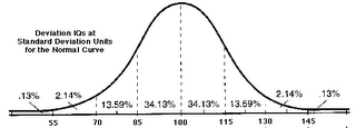
Deviation IQ Scores, sometimes called Wechsler IQ scores, are a standard score with a mean of 100 and a standard deviation of 15. We can thus see that the average IQ for the general population would be 100. If IQ is normally distributed, we would expect that two-thirds (68.26%) of the population would have deviation IQ's between 85 and 115. That is because 85 is one standard deviation below the mean and 115 is one standard deviation above the mean. We would expect that 99.72% of the distribution would lie within three standard deviations of the mean (that is IQs between 55 and 145).

The Stanford-Binet Scale of Intelligence IQ is also a standard score with a mean of 100 but with a standard deviation of 16. Thus a Wechsler IQ of 115 (one SD above the mean) would be equivalent to a Binet IQ of 116 (also one SD above the mean). A Wechsler IQ of 130 (two SDs above the mean) would be equivalent to a Binet IQ of 132. In some definitions of mental retardation, the cut off for an IQ score indicative of mental retardation is set at two standard deviations below the mean of the general population. This would be equivalent to a Wechsler IQ of 70 but a Stanford-Binet IQ of 68. We would also expect that 2.27% (.13% + 2.14% = 2.27%) of the population would have IQs this low.

Z-Scores
When a score is expressed in standard deviation units, it is referred to as a Z-score. A score that is one standard deviation above the mean has a Z-score of 1. A score that is one standard deviation below the mean has a Z-score of -1. A score that is at the mean would have a Z-score of 0. The normal curve with Z-scores along the abscissa looks exactly like the normal curve with standard deviation units along the abscissa.

Percentile Ranks
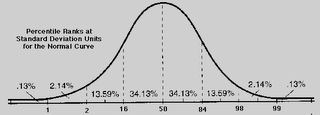
Another useful derived score is the percentile rank. The percentile rank is the percentage or proportion of scores that score lower than a given score. If you received a percentile rank of 90 then 90% of the scores would be lower than your score and 10% of the scores would be higher. You could also say that your score is at the 90th percentile. The median for any set of scores (by definition) is at the 50th percentile. That is, 50% of the scores are lower than the median, and 50% of the scores are higher than the median. Ordinarily percentiles are reported as whole numbers so the highest percentile possible would be 99 and the lowest possible would be 1. A score that is one standard deviation below the mean would have a percentile rank of 16 (0.13 + 2.14 + 13.59 = 15.86). A score that is two standard deviations below the mean would have a percentile rank of 2 (0.13 + 2.14 = 2.27). A score that was three standard deviations below the mean would be at the 1st percentile and one that was three standard deviations above the mean would be at the 99th percentile. Some test designers have used the concept of extended percentile ranks to make finer divisions for scores at the upper half of the 99th percentile and at the lower half of the 1st percentile.

T-Scores
Another commonly used derived scores based on the normal curve, is the T-score. T-scores are derived scores with a mean of 50 and a standard deviation of 10. The average T-score for a group of scorers would be 50. We can see that a T-score of 60 would be equivalent to a Z-score of 1, and a Deviation IQ score of 115. Each of these scores would be one standard deviation above the mean and would be equal to or higher than 84.13% of the scores (50.00% + 34.13% = 84.13%)

http://www-stat.stanford.edu/~naras/jsm/NormalDensity/NormalDensity.html

Lessons: Continuation - Inferential Statistical Tests

Click the Below Link to Progress to the Next Set of Lessons.

1. Hypothesis Testing
2. t-tests
3. z-test
4. ANOVA
5. Chi Squared
6. Probability

http://statstestsedresearch.blogspot.com/